
Introduction to the Boon Nano
The Boon Nano is a high-speed, high-efficiency, clustering and segmentation algorithm based on unsupervised machine learning. The Nano builds clusters of similar n-space vectors (or patterns) in real-time based on their similarity. Each pattern has a sequence of features that the Nano uses in its measurement of similarity.
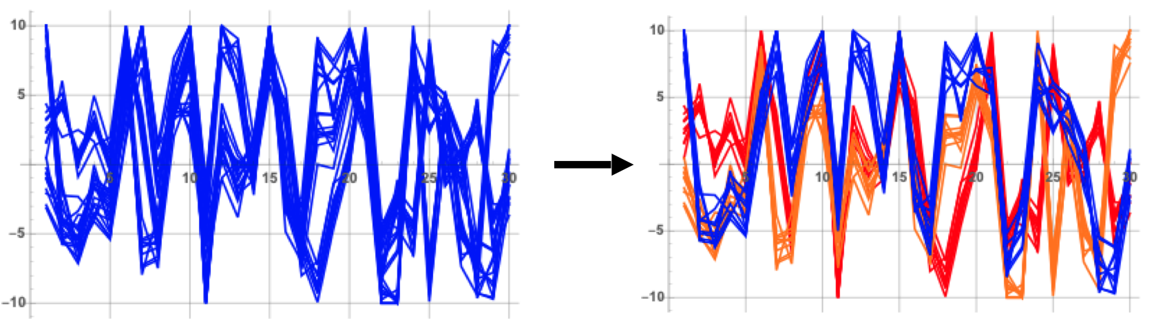 |
| Figure 1: Semi-structured data is segmented by the Boon Nano based on L1-distance similarity. |
Examples of Patterns
- Servo-Motor Tags: Industrial motors are controlled by servo feedback loops that have multiple features. A pattern that could be used to build an ML model of motor performance date might be (Output Current, Torque Trim, Position, Velocity, Position Error, Velocity Error)
- Flight Recorder Data: An aircraft has multiple sensors that define its operating state at any point in time. For example, a pattern might have these features (Altitude, Air Speed, Ground Speed, Lateral Acceleration, Longitudinal Acceleration, Vertical Acceleration, Left Aileron Position, Right Aileron Position)
- Power Spectra: The output of vibrational sensors is often transformed into frequency spectra. In this case, the features represent adjacent frequency bands, and the value of each feature is the power from the source signal in that frequency band.
- Triggered Impulsive Data: If n consecutive samples from a single sensor are acquired like a snap shot, they can be compared by shape and clustered by similarity to gain insight about the varieties of signals occurring in the data stream. The snap shot is typically triggered by a threshold crossing of the signal.
- Single-Sensor Streaming Data: Consecutive overlapping windows of the most recent n samples from a sensor form a natural collection of n-dimensional vectors.
- Histogram of Magnitudes: This common technique from computer vision builds, for each pixel, a histogram of the grayscale values of the surrounding pixels. If values range from 0 to 255, then these patterns might have 256 featues. Then an image is transformed into a large collection of patterns (one for each pixel) that can be processed through the Boon Nano.
Using the Boon Nano
The Boon Nano clusters its input data by assigning to each pattern an integer called its cluster ID. Patterns assigned the same cluster ID are similar in the sense of having a small L1-distance from each other. The similarity required for patterns assigned to the same cluster is determined by the percent variation setting and the configured feature ranges (described below). Sometimes a pattern is processed by the Nano that is not similar to any of the existing clusters. In this case, one of two actions is taken. If learning mode is on and if the maximum allowed clusters has not been reached, the pattern becomes the first member of a new cluster and the number of clusters in the model increases by one. If learning mode is off or the maximum number of clusters has been reached, the pattern is assigned the special cluster ID 0. There is no assumption that can be made about the similarity of pattern assigned to cluster 0, but they are all known to be significantly different from the non-zero clusters in the existing model. This dynamic learning process of assigning patterns to existing clusters or, if needed, creating new clusters is called training a model.
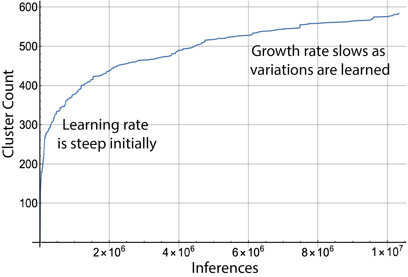 |
| Figure 2: The number of clusters grows quickly as the first patterns from the input data are processed. The slope of the growth curve levels off as the model matures and as nearly all incoming patterns already have a cluster to which they can be assigned. |
The Boon Nano is deployed in both a general-use platform called Expert Console and as a streaming sensor analytics application called Amber
- Expert Console: The Expert console provides the full functionality of the Boon Nano including all analytics (described below) and is oriented toward batch processing of input data.
- Amber: Amber is a specialized interface for the Nano designed for real-time streaming data. Amber provides an easy-to-use interface for sending streams of successive sensor values as a time series and getting back analytic values that correspond one-for-one to the sensor values. These analytic values are typically used for anomaly detection in the sensor stream.
Configuring the Boon Nano
Clustering Configuration
The Boon Nano uses the clustering configuration to determine the properties of the model that will be built for the input data.
- numericType: One numeric type is chosen to apply to all of the features in each input vector. A good default choice for numeric type is float32, which represents 32-bit, IEEE-standard, floating-point values. In some cases, all features in the input data are integers ranging from -32,768 and 32,767 (int16) or non-negative integers ranging from 0 to 65,535 (uint16), for instance, bin counts in a histogram. Using these integer types may give slightly faster inference times, however, float32 performance is usually similar to the performance for the integer types. For nearly all applications, float32 is a good general numeric type to use.
- Feature List: A pattern is comprised of features which represent the properties of each column in the vectors to be clustered. Each feature has a range (a min and max value) that represents the expected range of values that feature will take on in the input data. This range need not represent the entire range of the input data. For example, if the range of a feature is set to -5 to 5, then values greater than 5 will be treated as if they were 5 and value less than -5 will be treated as -5. This truncation (or outlier filtering) can be useful in some data sets. Each feature is also assigned a weight between 0 and 1000 which determines its relative importance in assignment of patterns into clusters. Setting all weights to 1 is a common setting, which means all features are weighted equally. Setting a weight to 0 means that feature is ignored in clustering as if it were not in the vector at all. Finally, each feature can be assigned an optional user-defined label (for example, “systolic”, “pulse rate”, “payload length”, “output current”). Labels have no effect on the clustering.
- percentVariation: The percent variation setting ranges from 1.0% to 20.0% and determines the degree of similarity the Nano will require between patterns assigned to the same cluster. Smaller percent variation settings create more clusters with each cluster having more similarity between patterns assigned it. A larger choice for percent variation produces coarser clustering with fewer clusters.
- streamingWindowSize: This indicates the number of successive samples to use in creating overlapping patterns. For instance, it is typical in single-sensor streaming mode applications to have only one feature and a streaming window size greater than 1. If there is one feature, and the streaming window size is 25, then each pattern clustered by the Nano is comprised of the most recent 25 values from the sensor. In this case, each pattern overlaps 24 samples with its predecessor. In batch mode, it is typical to use a streaming window size of 1. (See Amber for additional details.)
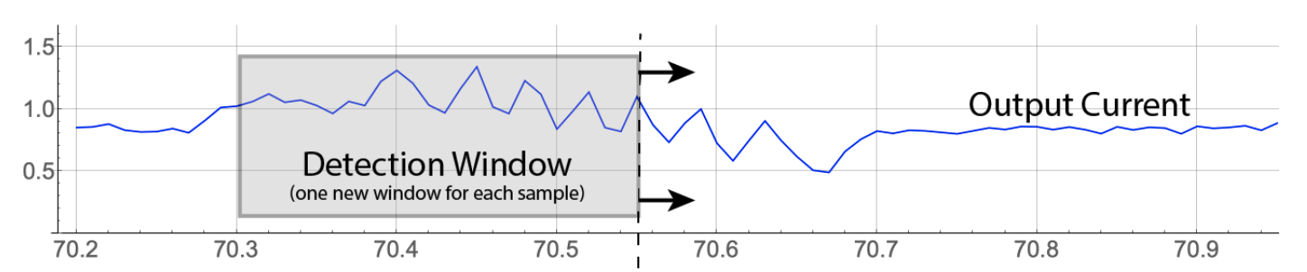 |
| Figure 3: One feature (all samples from the same sensor) and streaming window size of 25. Each input vector is 25 successive samples where we form successive patterns by dropping the oldest sample from the current pattern and appending the next sample from the input stream. |
Autotuning Configuration
Two clustering parameters, the percent variation and the range for each feature, can be autotuned, that is, chosen automatically, by the Boon Nano prescanning representative data. The range for each feature can be autotuned either individually or a single range can be autotuned to apply to all features.
One of the most difficult parameters to configure in unsupervised machine learning is the desired number of clusters needed to produce the best results (as with K-means) or (in the case of the Boon Nano) the desired percent variation to use. This is because one would not generally know a priori the underlying proximity structure of the input vectors to be segmented.
To address this, the Boon Nano can automatically tune its percent variation to create an balanced combination of coherence within clusters and separation between clusters. In nearly all cases, autotuning produces the best value for the percent variation setting. However, if more granularity is desired you can lower the percent variation manually. Similarly, if the autotuned percent variation is creating too much granularity (and too many clusters) then you can choose to manually increase the percent variation above the autotuned value.
- autotuneRange: If this parameter is set to true, the user-supplied range(s) specified in the Nano configuration gets replaced with the autotuned range. If set to false, the user-supplied range(s) is left intact.
- autotunePV: If this parameter is set to true, the user-supplied percent variation specified in the Nano configuration get replaced with the percent variation found through the autotuning. If set to false, the user-supplied percent variation is left intact.
- autotuneByFeature: If this is set to true and the option to autotune the range is set to true, then the autotuning will find a range customized to each feature. If false, then autotuning will find a single range that applies to all features.
- exclusions: An array of exclusions may be provided which causes the autotuning to ignore those features. For instance, if the array [2 7] is provided, then autotuning is applied to all features except the 2nd and 7th features. An empty exclustions array, [ ], means that no features will be excluded in the autotuning.
Clustering Results
When a single pattern is assigned a cluster ID, this is called an inference. Besides its cluster ID, a number of other useful analytic outputs are generated. Here is description of each of the ML-based outputs generated by the Boon Nano in response to each pattern.
Cluster ID (ID)
The Boon Nano assigns a Cluster ID to each input vector as they are processed. Following configuration of the Nano, the first pattern is always assigned to a new cluster ID of 1. The next pattern, if it is within the defined percent variation of cluster 1, is also assigned to cluster 1. Otherwise it is assigned to a new cluster 2. Continuing this way all patterns are assigned cluster IDs in such a way that each pattern in each cluster is within the desired percent variation of that cluster’s template. In some circumstances the cluster ID 0 may be assigned to a pattern. This happens, for example, if learning has been turned off or if the maximum cluster count has been reached. It should be noted that cluster IDs are assigned serially so having similar cluster IDs (for instance, 17 and 18) says nothing about the similarity of those clusters. However, a number of other measurements described below can be used to understand the relation of the pattern to the model.
In some conditions, a negative cluster ID may be assigned to a pattern. A negative ID indicates that the pattern is not part of the learned model, but the Boon Nano can still give information about the pattern as it relates to the learned model. This can be especially useful for anomaly detection where a pattern falls outside the model. In this case Root Cause Analysis using the negative cluster ID will provide additional information about the reason the pattern is outside the model. (See Root Cause Analysis below.)
Operational Mode (OM)
Although cluster IDs do not indicate anything about relative proximity of clusters in n-dimensional space, in many situations the sequence of cluster IDs that are being assigned to successive patterns will indicate a standing operating state of the data source generating the patterns (for example, sensor telemetry from a motor running for hours at a set speed). We derive the Operational Mode value by computing the average of the most recent cluster IDs. The OM value can be used to identify significant changes in operational state of the data source. A significant change in OM value indicates that something has changed in the recent sequence of cluster IDs. For example, a motor running at 10% and then increasing at 50% will show a discrete shift in OM value. Conversely, OM values can be used across time to link states of the data source that are likely to be the same. For example, a motor running at 10%, then 50%, and then back to 10% will show a discrete shift in OM from the 10% mode to the 50% mode and then back to the 10% mode. This converse approach must be use with caution, as it is possible, but unlikely, that two different operational states of a data source could have the same OM value.
Two Anomaly Axes
The Boon Nano can measure anomalies along two different axes: frequency and distance. Together these two axes capture the full scope of what may be considered as an “anomaly” within a set of input patterns.
- Frequency Anomalies: This is the common meaning people assign to the word “anomaly”, that is, a pattern that occurs very rarely among all patterns in the input set. It could perhaps better be called an infrequency anomaly, as it is the kind of anomaly that indicates a pattern that occurs only very infrequently.
- Distance Anomalies: This is a pattern that is very different from the model in terms of n-dimensional distance without any reference to whether it is occurring frequently or infrequently.
Raw Anomaly Index (RI) (Frequency Anomaly)
The Boon Nano assigns to each pattern a Raw Anomaly Index, that indicates how many patterns are in its cluster relative to other clusters. These integer values range from 0 to 1000 where values close to zero signify patterns that are the most common and happen very frequently. Values close to 1000 are very infrequent and are considered more anomalous the closer the values get to 1000. Patterns with cluster ID of 0 have a raw anomaly index of 1000.
Smoothed Anomaly Index (SI) (Frequency Anomaly)
Building on the raw anomaly index, we create a Smoothed Anomaly Index which is an edge-preserving, exponential, smoothing filter applied to the raw anomaly indexes of successive input patterns. These values are also integer values ranging from 0 to 1000 with similar meanings as the raw anomaly index. In cases where successive input patterns do not indicate any temporal or local proximity, this smoothing may not be meaningful.
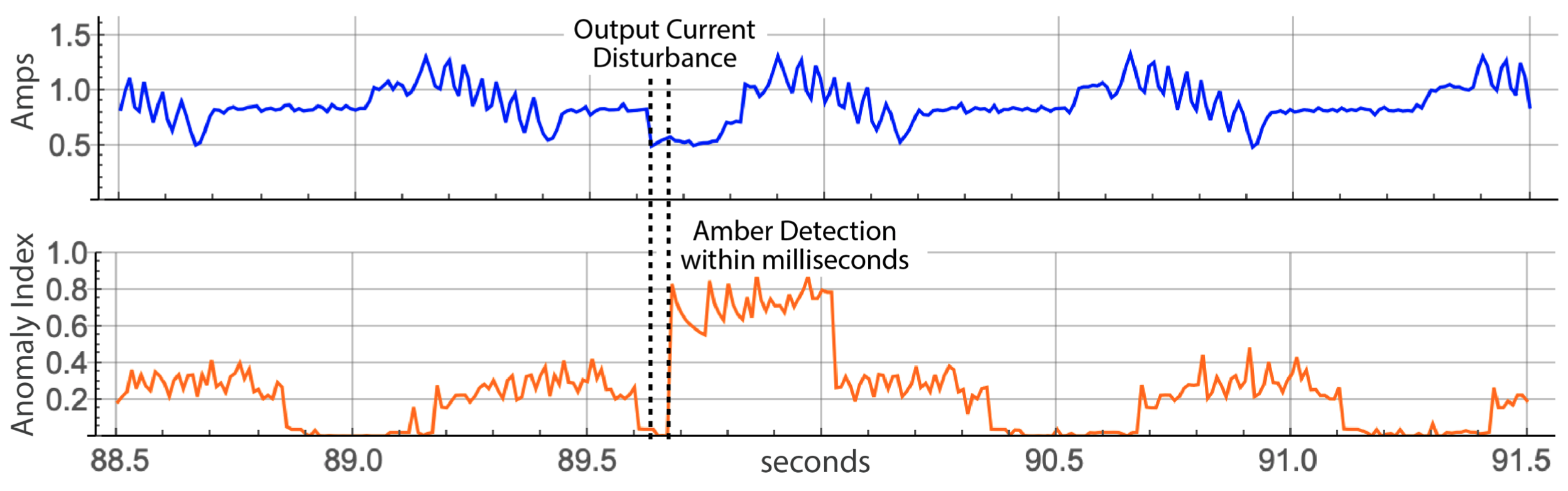 |
| Figure 4: Raw sensor signal (Blue) and SI, the Smoothed Anomaly Index (Amber), showing a rarely occuring pattern in the sensor stream model. |
Frequency Index (FI) (Frequency Anomaly)
Similar to the anomaly indexes, the Frequency Index measures the relative number of patterns placed in each cluster. The frequency index measures all cluster sizes relative to the average size cluster. Values equal to 1000 occur about equally often, neither abnormally frequent or infrequent. Values close to 0 are abnormally infrequent, and values significantly above 1000 are abnormally frequent.
Distance Index (DI) (Distance Anomaly)
The Distance Index measures the distance of each cluster template to the centroid of all of the cluster templates. This overall centroid is used as the reference point for this measurement. The values range from 0 to 1000 indicating that distance with indexes close to 1000 as indicating patterns furthest from the center and values close to 0 are very close. Patterns in a space that are similar distances apart have values that are close to the average distance between all clusters to the centroid.
Novelty Index (NI) (Combined Distance and Frequency Anomaly)
The Novelty Index measures along both anomaly axes in one value. The values range from 0 to 1000 with the following interpretations.
- NI equal to 0: The pattern is found in the model.
- NI close to 0: The pattern is not in the model, but it is very close to a large cluster in the model.
- NI close to 500: The pattern is not in the model, but it is either very close to a small cluster in the model or relatively close to a large cluster in the model.
- NI close or equal to 1000: The pattern is not in the model, and it is at least a full percent variation from the closest cluster in the model.
Practically speaking, NI values close to 0 indicate a non-anomalous pattern. As the NI grows toward 1000, it indicates increasing non-compliance or non-alignment of patterns relative to the trained model.
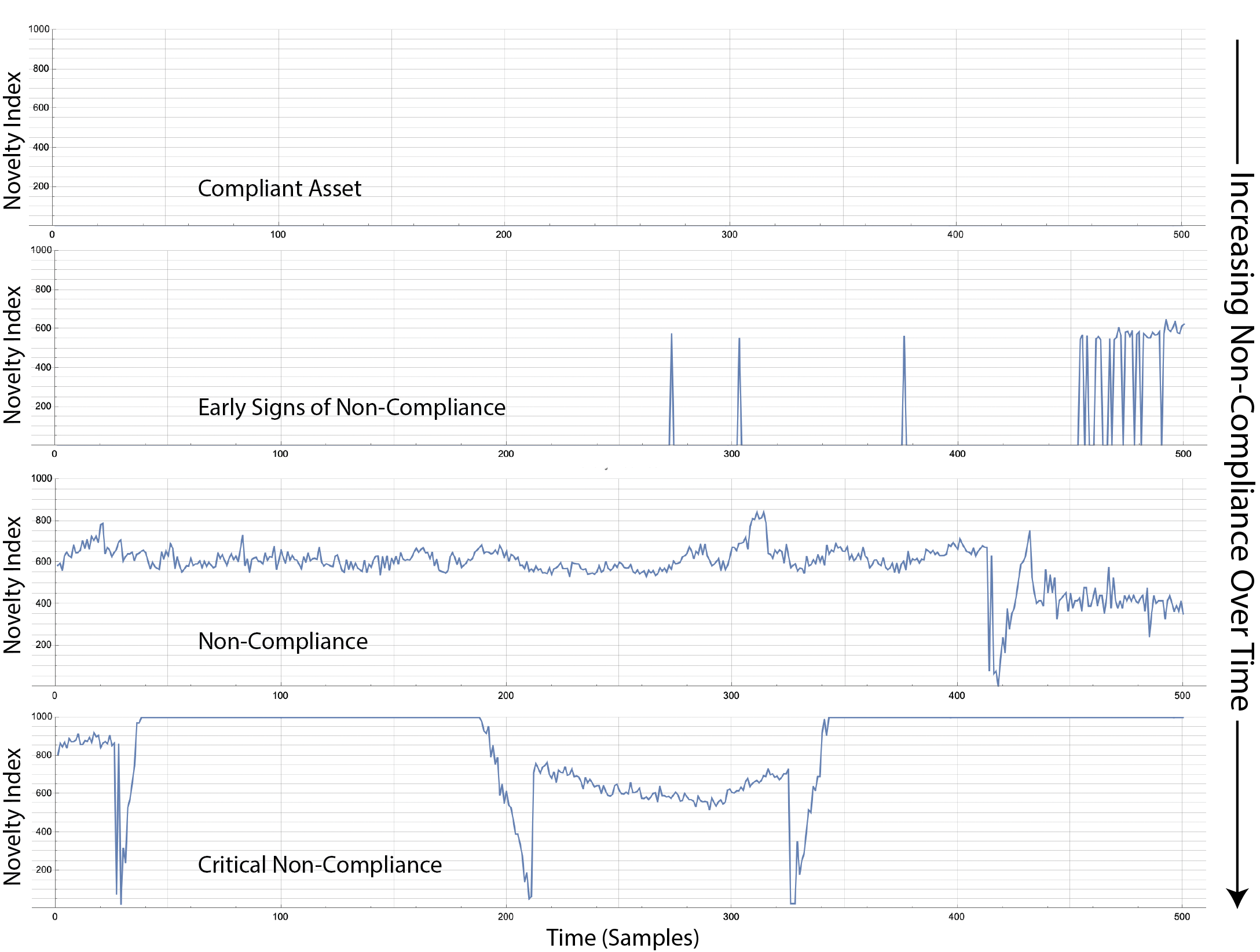 |
| Figure 5: Novelty Index of an industrial robot measuring current from 6 joints as a single 6-feature pattern. Over time the Novelty Index increases from 0 (fully compliant relative to training) and shows increasing non-compliance as the asset wears toward a maintenance event. |
Smoothed Novelty Index (NS) (Combined Distance and Frequency Anomaly)
The Smoothed Novelty Index is the exponentially smoothed sum of recent novelty indexes (NI). As such it is suited for time-series where a single spike in the NI value may not be significant but where a trend of increasing NI values indicate increasing non-compliance of patterns relative to the model.
Root Cause Analysis (RC)
Each processed pattern is assigned a cluster ID. The Boon Nano associates each ID with an associated Root Cause vector. This vector has the same number of values of the number of features in patterns of the model. Each value in the vector is a representation of each feature’s significance in the cluster to which it was assigned. Values range from 0 to 1 where relatively high values indicate features that are more influential in the creation of the cluster. Values close to 0 lack statistically significance and no conclusion can be drawn from them. This is especially important for anomaly detection where the RCA vector can be used to determine which features are implicated in a detected anomaly (Figure 6).
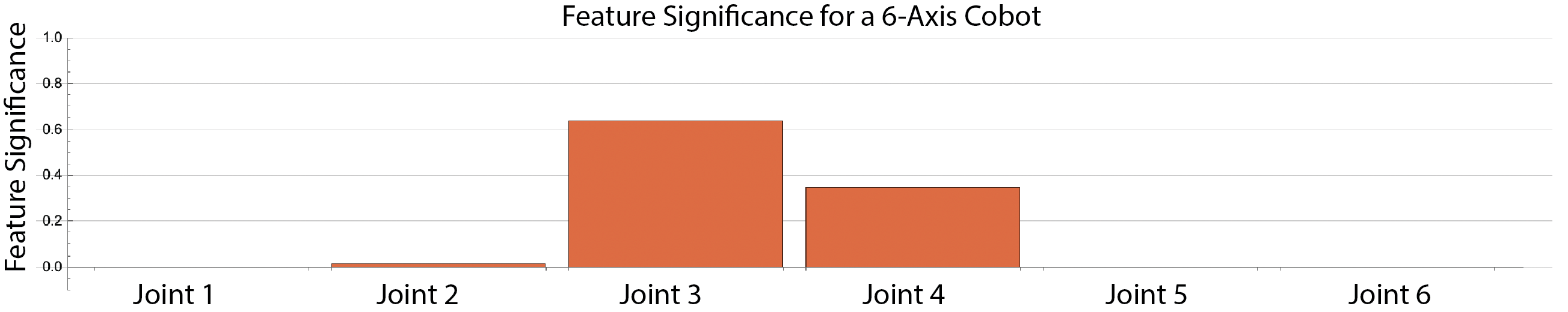 |
| Figure 6: The RCA vector shown in the figure was from a 6-joint cobot running a 3-position motion profile. The Novelty Index for one pattern was near 600 as shown in Figure 5. This NI value was returned along with a negative cluster ID. The RCA vector for this negative ID indicates that joints 2 and 3 are implicated in this anomaly. |
Nano Status: Information about the Nano Model
While Nano Results (previous section) give specific analytic results for the patterns in the most recently processed sample buffer, Nano Status provides core analytics about the Nano model itself has been constructed since the Nano was configured. The status information is indexed by cluster ID beginning with cluster 0.
anomalyIndexes
The values in this list give raw anomaly index (RI) for each cluster in the Nano’s current model. The cluster assigned the most patterns has anomaly index of 0 up to a maximum of 1000 for a cluster that has only been assigned one pattern. Cluster 0 always has anomaly index of 1000.
-
clusterSizes: The values in this list give the number of patterns that have been assigned to each cluster beginning with cluster 0. When learning is turned off, this value does not change.
-
totalInferences: This is the total number of patterns successfully clustered. The total of all the values in clusterSizes should also equal this value.
-
anomalyIndexes: The values in this list give raw anomaly index (RI) for each cluster in the Boon Nano’s current model. The cluster assigned the most patterns has anomaly index of 0 up to a maximum of 1000 for a cluster that has only been assigned one pattern. Cluster 0 always has anomaly index of 1000.
-
frequencyIndexes: Similar to the anomaly indexes, each value in this list gives the frequency index associated with the corresponding cluster whose ID beginning with cluster 0. These values are integers that range from 0 and up. While there is no definitive upper bound, each Nano model will have a local upper bound. Values below 1000 indicate clusters whose sizes are smaller than average, where 0 is the most common cluster size. Values above 1000 have been assigned more patterns than average and the further they are above 1000, the larger the cluster is. This statistic is a dual use value where anomalies (very small and very large) can be considered when they have values on either side of 1000.
-
distanceIndexes: Distance indexes refer to each cluster’s spatial relation to the other clusters. Values close to 1000 are very far away from the natural centroid of all of the clusters. Values close to 0 are located near the center of all the clusters. On average, these values don’t vary much and develop a natural mean. This is also a dual threshold statistic since the natural mean represents the typical spacing of the clusters and there can be abnormally close clusters and abnormally distant clusters.
-
clusterGrowth: The cluster growth curve shows the number of inferences between the creation of each new cluster (Figure 2). The list returned by clusterGrowth is the indexed pattern numbers where a new cluster was created which can be used as the x-values of this curve. The y-values can be derived as an ascending sequence of cluster IDs: 0, 1, 2, 3, etc. For instance, if clusterGrowth returns [0 1 5 7 20], the coordinates of the cluster growth plot would be: [0 0], [1 1], [5 2], [7 3] [20 4].
-
PCA: Clusters in the Boon Nano are naturally mapped into a very high-dimensional space. This makes it difficult to meaningfully visualize the clusters on a two- or three-dimensional plot. The Nano’s PCA list is similar to traditional principal component analysis in the sense it can be used to remap a high-dimensional vector into a lower dimensional space that, as far as possible, preserves distances and limits the flattening effects of projection. The PCA coordinates can be used, for example, to assign RGB values to assign a meaningful color to each cluster. Clusters with different but similar colors are from clusters whose assigned patterns are different enough to be in distinct clusters but that are still close to each relative to the other clusters in the model. The zero cluster is always the first value in the list of PCA values and is represented by [0, 0, 0].
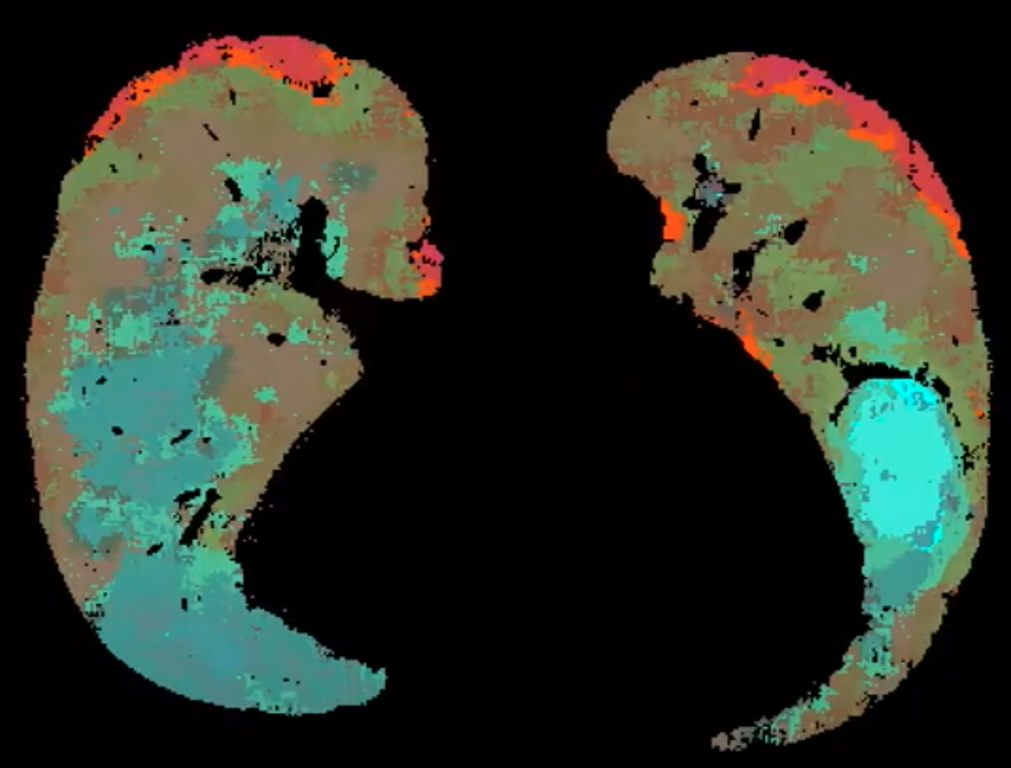 |
| Figure 7: Pulmonary CT image using PCA coloring to show distinct tissue textures and the gradients between them. |
-
numClusters: This is a single value that is the current number of clusters in the model including cluster 0. This value should equal the length of the lists: PCA, clusterSizes, anomalyIndexes, frequencyIndexes, distanceIndexes, clusterGrowth.
-
averageInferenceTime: The value returned here is the average time to cluster each pattern in microseconds.
Example
We now present a very simple example to illustrate some of these ideas. A set of 48 patterns is shown in the figure below. A quick look across these indicates that there are at least two different clusters here. Each pattern has 16 features so we configure the Nano for
- Numeric Type of float32
- Pattern Length of 16
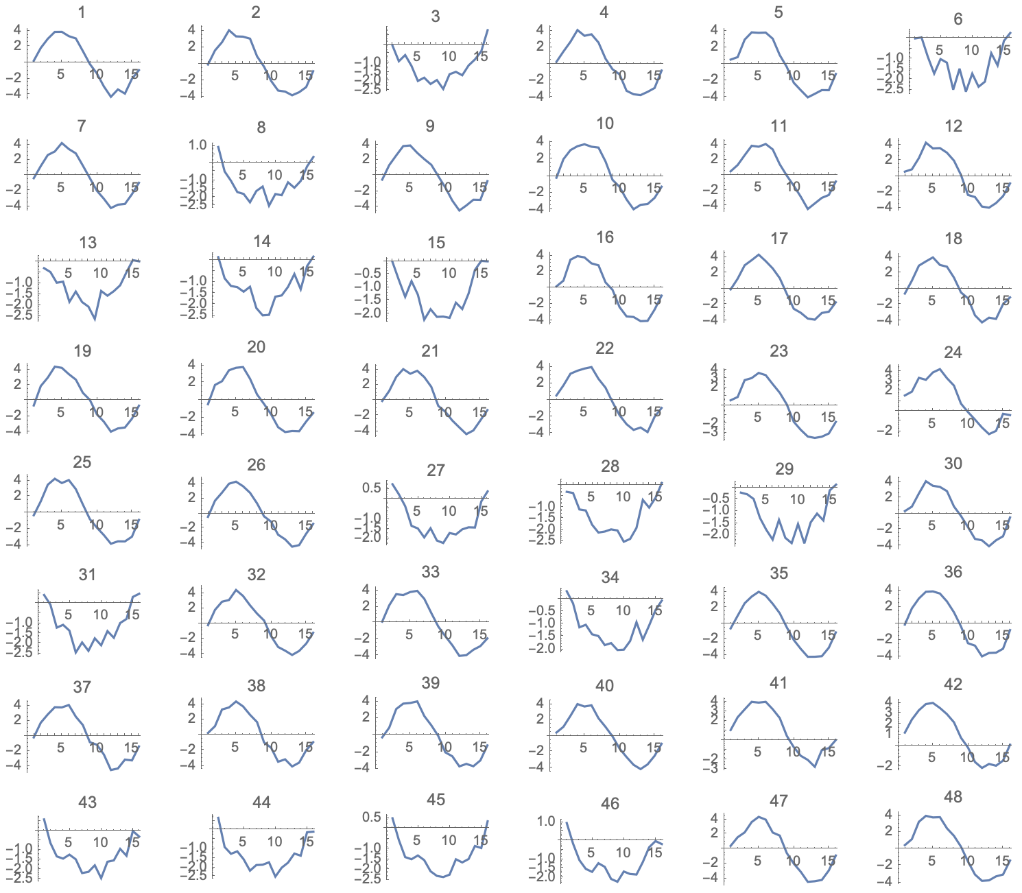 |
| Figure 8: A collection of 48 16-dimensional vectors to be clustered |
We could select the mininum and maximum by visual inspection, but it is not possible to determine the correct Percent Variation this way. So we instead load the patterns into the Nano and tell the Nano to Autotune those parameters. The results comes back with:
- Min = -4.39421
- Max = 4.34271
- Percent Variation = 0.073
We configure the Nano with these parameters and then run the patterns through the Nano, requesting as a result the “ID” assigned to each input pattern. We receive back the following list: {1, 1, 2, 1, 1, 2, 1, 2, 1, 1, 1, 1, 2, 2, 2, 1, 1, 1, 1, 1, 1, 1, 1, 3, 1, 1, 2, 2, 2, 1, 2, 1, 1, 2, 1, 1, 1, 1, 1, 1, 3, 3, 2, 2, 2, 2, 1, 1}
Comparing this to the sequence in the figure, we see that this is a reasonable clustering assignment. Further, we see that there is a third cluster that may have been missed by our intuitive clustring. This cluster had just three patterns assigned to it. The figure below shows the waveforms plotted on the same axes and colored according according to their assigned cluster IDs.
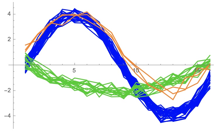 |
| Figure 9: 48 patterns colored according to their assigned clusters |
The Raw Anomaly index for each of the three clusters are as follows:
- Cluster 1 Raw Anomaly Index: 0
- Cluster 2 Raw Anomaly Index: 170
- Cluster 3 Raw Anomaly Index: 563
This indicates Cluster 1 had the most patterns assigneed to it. Cluster 2 was also common, and Cluster 3 was significantly less common. It is worth noting that a Raw Anomaly Index of 563 would not be sufficient in practice to indicate an anomaly in the machine learning model. Typically, useful anomaly indexes must be in the range of 700 to 1000 to indicate a pattern that is far outside the norm of what has been learned.
Simplification Disclaimer: This is an artificially small and simple example to illustrate the meaning of some of the basic principles of using the Boon Nano. In particular:
- The Boon Nano is typically be used to cluster millions or billions of patterns.
- The number of clusters created from “real” data typically runs into the hundreds or even thousands of clusters.
- The speed of the Boon Nano for such a small data set is not noticeable over other clustering techniques such as K-means. However, when the input set contains 100s of millions of input vectors or when the clustering engine must run at sustained rates of 100s of thousands of inferences per second (as with video or streaming sensor data), the Boon Nano’s microsecond inference speed makes it the only feasible technology for these kinds of applications.